4 Reproducible research

4.1 Introduction

This series introduces computational reproducibility and its importance to modern research. We will teach the general principles for reproducible computer-based analyses, along with specific methods and tools for reproducibility with RStudio. We will also introduce version control with GitHub, an essential tool in a team environment.

You will learn how to:

• Construct reproducible, automatable workflows in R.
• Create reproducible documents using R Markdown to include underlying code/computations with relevant graphical and statistical results in several different formats (reports, presentation slides, handouts, notes).
• Use Git version control.
• Integrate version control with GitHub for both personal and group projects.

This intermediate workshop series assumes prior experience with R (such as that in our Introduction to R workshop).

Please call a TA if you have any problems executing the code or need any help with the exercises.

4.1.1 Formatting

In text-paragraphs, code is always formatted with a monospace font and surrounded by a box, like this. Longer examples of code will be in their own separate box.

First line of code
Second line of code
...

In many cases the output for code in these boxes will be below them.

Replace any placeholder indicated by angular brackets <placeholder> with your own code.

Pressing a Key on the keyboard is formatted like that.

4.2 Before the workshop

4.2.1 Setup Instructions

Please come to the workshop with your laptop set up with the required software and data files described in our setup instructions.

4.2.2 Background

Please read Hallam SJ et al. 2017. Sci Data 4: 170158 “Monitoring microbial responses to ocean deoxygenation in a model oxygen minimum zone” to learn more about the data used in this workshop. You can also check out this short video showing the sampling process!

4.3 Terminology

Reproducibility is purported to be at the heart of science. But what do we mean when we say “reproducible research”? Researchers generally think of replicating an experiment and obtaining the same result (direct replicability). However, what we should actually strive for is true reproducibility, reaching the same conclusions through different methods. Moreover, we usually think of the reproducibility of wet-lab experiments. It is a somewhat newer movement for researchers to make analysis and computational methods reproducible.

In this workshop, we are working toward is repeatability, the ability to repeat a computational analysis exactly. These methods can then be built upon by other researchers or yourself to find true reproducibility.

4.4 Why reproducibility?

It helps you remember what you did.

Your closest collaborator is you six months ago. And past you doesn’t answer email. ~ Karl Broman, UW-Madison

Even if no other human ever reads your code, it is worth making it reproducible for your future self. It is like a classical lab notebook. You wouldn’t expect yourself to remember how many ng of DNA you used in a PCR reaction two weeks ago, right? So, you shouldn’t expect yourself to remember exact computational workflows.

It prevents human error.

If you do anything by hand once, you’ll likely do it a hundred times… and five of those times, you’ll make a mistake. The easiest solution is to let a computer complete the repetitive tasks. So, this means you should NOT do anything analysis-related with a mouse (*cough* Excel *cough*).

It helps you communicate with others.

Past you may be your closest collaborator, but you likely have other people you work with, and you probably want to communicate your science to the larger scientific community at some point (#PublishOrPerish). Making your code reproducible makes it accessible to others for their understanding of your research as well as potentially for their use in their own work.

It is faster.

This almost goes without saying because a computer can do pretty much anything computationally faster than a human. But also, speed comes with repetition. If your code, report, slides, etc., are reproducible, then when you need to make a small change or produce a similar document in the future, that can be done quickly and with minimal effort on your part.

4.5 R projects

One of the most common hurdles to code reproducibility is file paths. If you have all your code and data in ~/Documents and someone copies it all to their ~/Desktop, then any links to files in your code will be broken. For example, read.table(file = "~/Documents/mydata.csv") will not work for the other person because they do not have that file in that place.

The level 1 solution to this is to start your code by setting the working directory like

setwd("~/Documents")

Thus, others need only change this one line of code to use your script.

But we can do one better in R by eliminating the need for any file paths with R projects. RStudio creates an .Rproj file that links all of your files and outputs to the project directory when you create a project. When you import data, R automatically looks for the file in the project directory instead of you having to specify a full file path on your computer like ~/Documents. R also automatically saves any output to the project directory. Finally, projects allow you to save your R environment in .RData so that when you close RStudio and then re-open it, you can start right where you left off without re-importing any data or re-calculating any intermediate steps.

RStudio has a simple interface to create and switch between projects, accessed from the button in the top-right corner of the RStudio window. (Labelled “Project: (None)” initially.)

Let’s create a project to work in for this workshop. Start by clicking the “Project” button in the upper right or the “File” menu. Select “New Project,” and the following will appear.

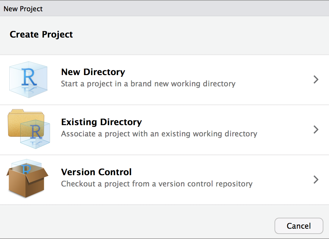
You can either create a project in an existing directory or make a new directory on your computer - just be sure you know where it is.

After your project is created, navigate to its directory using your Finder/File Explorer, and you will see the .RProj file.

To access this project in the future, simply double-click the .RProj file, and RStudio will open the project or choose File > Open Project from within an already open RStudio window.

4.6 R scripts

The next level of reproducibility in R is to use R scripts. You should never input commands into the R console because they are not saved there. Instead, input them into an R script and run them from the script. Then, you have a record of all the steps you performed in an analysis.

Well… not actually never. If you’re using R as a fancy calculator, you’re probably okay to perform some math in the console. And you likely don’t want to save the time you use the help function ?. But pretty much everything else should go in a script.

Let’s practice this.

Create a new R script under File > New File > R script and input the following code.

# Load packages
# Suite of packages for data manipulation and visualization
library(tidyverse)

# Load data from our GitHub
dat <- read.csv("https://raw.githubusercontent.com/EDUCE-UBC/educer/main/data-raw/data_intro_ws.csv")

# Create plot of oxygen by depth
O2_plot <- quickplot(data = dat,
                     x = O2_uM,
                     y = Depth_m,
                     color = Season,
                     main = "Saanich Inlet: Seasonal oxygen depth profile")

# Save plot
ggsave("O2_plot.png")

Save the file under the name O2_plot.R.

Now we can execute our workflow in a couple of different ways. We can

1. open it in RStudio and run it.
2. source it from the R console with source("O2_plot.R").
3. run it from the terminal.

4.6.1 Running an R script from the terminal

4.6.1.1 What is a terminal?

If you are not familiar with the terminal, it may be daunting at first. To understand the purpose of the terminal, it helps to understand what it is.

To communicate with your operating system, you interact with a user interface. The user interface is also called the shell (because it is your computer’s “outer layer”– the part that you can see and interact with). Most frequently, the user interface is visual: it consists of icons that you can click on, windows that you can re-size, a desktop on which you can put files, and so on. This kind of shell is called a graphical user interface, or GUI. Alternatively, you can interact with the operating system using a text-based interface: you navigate your computer and execute programs by spelling out commands. This kind of shell is called a command-line interpreter, or CLI.

Some operating systems (including Linux and macOS) belong to a family of operating systems called Unix. There are different text-based Unix shells, but the most famous is called Bash. (The name is a pun: it means Bourne again shell because it is a more recent version of an older shell called Bourne shell.) We access Bash via a program on your computer called the terminal.

Windows operating systems also have a command-line shell, called the Command Prompt. However, most command-line software (e.g. Git) is optimized for Bash, so we encourage Windows users to use a terminal emulator such as GitBash.

4.6.1.2 How to navigate your computer using the terminal

When you use the GUI, you can visually navigate your computer by opening directories, which you do by double-clicking icons shaped like folders. How do you navigate your computer using the terminal?

Start by opening the terminal (or GitBash if you are using Windows). The first question you might ask yourself is, “where am I right now?”, i.e. what folder are you located in? You can ask the terminal what the current folder is by typing pwd, followed by Return (Enter). pwd stands for print working directory. You will see the absolute path to the current folder.

You may also wonder, “what directories and files are located in the current directory?”. You can access this information with the command ls, which will list all the files.

If you want to navigate into one of the directories listed in the previous step, you can do so by typing cd, followed by a space, followed by the directory’s name. For example, if you are on a Mac and your current working directory is /Users/<your username>, you can navigate to the Documents folder by typing cd Documents.

Note: If the directory you want to access has a space in its name, you need to write a backslash \ before the space, e.g. cd My\ Documents.

If you want to navigate out of a directory, you can type cd .., which will return you to the parent directory.

4.6.1.3 How to run your R script using the terminal

Now that you know how to navigate your computer using the terminal navigate to your project directory. Once you’ve done so, type Rscript O2_plot.R and press Enter.

If you scripted our workflow right, running the script will produce the O2_plot.png file in your project directory. We can re-run it multiple times (try it after deleting the plot), always recreating the output. Congratulations, you’ve automated your workflow!

4.6.2 Modularizing by task

Keeping all of our analysis in one file is okay for a small example like this. However, extensive analyses should be broken up into multiple scripts, each completing one step (like data cleaning, statistical analysis, plotting, etc.) and saving the output to a file on your computer.

Then, you can create a driver script that is just a list of source commands calling all your individual scripts.

Why go through this extra effort? Modular scripts allow you to

• run individual steps manually if you need to.
• get intermediate results in files that you can look at, save, and share.
• execute another tool outside of R for a particular step in your workflow (e.g. python, Git, etc.).
• easily replace the driver with a full-blown workflow engine like Make (more on this later).

What would this look like for our example? The overall driver script would be

root_script.R

# load in data and packages
source("load.R")
# Create plot
source("plot.R")

And the individual step scripts could be

1. load.R

   # load data
   dat <- read.csv("https://raw.githubusercontent.com/EDUCE-UBC/educer/main/data-raw/data_intro_ws.csv")
   
   write.csv(dat, "data.csv")

   Note that we now need to save the data object to our computer with write.csv since it needs to be saved somewhere for use in the next script in the workflow.

2. plot.R

   # Load packages
   # Suite of packages for data manipulation and visualization
   library(tidyverse)
   
   # read in data
   dat <- read.csv("data.csv")
   
   # Create plot of oxygen by depth
   O2_plot <- quickplot(data = dat,
                        x = O2_uM, 
                        y = Depth_m, 
                        color = Season, 
                        main = "Saanich Inlet: Seasonal oxygen depth profile")
   
   # Save the plot
   ggsave("O2_plot.png")

   Note that loading the tidyverse package has been moved from the start of our single script to the beginning of the plot.R script. Packages need to be loaded in the script(s) using them, not yall at once in the first script in your workflow.

Now we can run our driver script in the terminal with Rscript root_script.R executing first load.R then plot.R, thus outputting the desired plot. You can easily see how this might scale up when you have dozens of scripts for a project!

4.6.3 Using Make

Make is an automation tool used to build executable programs and workflows. While it was initially designed to build software (like Linux), it is now widely used to manage projects with many input files and scripts that create several output files.

Make is language-independent; so, it can work with scripts for any program. Make is basically just one level more advanced than driver scripts in that it not only runs a list of scripts it also manages versions of all the associated files and keeps track of dependencies.

1. Make builds dependencies efficiently. If an input file hasn’t changed since its dependents were built, steps needed to create them don’t need to be executed. In contrast, a driver script will run all steps no matter what.

2. Make’s syntax provides documentation of your project’s workflow. Because you must list dependencies up-front in a Makefile, it’s easy to see what depends on what. This may not seem like a big deal in a straight pipeline as in our example, but once you have a web or network of dependencies, it’s a lot easier to visualize what’s going on by representing it this way.

3. Make is succinct. Make allows expressing dependency patterns (e.g. each .png file is produced from the data in file X.csv by running Rscript on the .R file of the same name), so that you don’t have to write out the recipe for building every single plot.

4. Make easily scales up. If down the line, you add another plot to the outputs produced by your workflow and use the same naming scheme, it will get picked up and automatically built the exact same way.

So how do we use Make?

We specify our workflow in a Makefile (note the capitalization). You can create this file in any text editor. It is best to work in the terminal with terminal-based text editors like nano, Emacs, etc. For this workshop, we will use RStudio as our text editor. However, please note that Make syntax is not the same as R. Tabs and spaces have very different and particular uses, as you will see below. To ensure that RStudio doesn’t replace your tabs with spaces, navigate Tools > Global Options > Code and ensure that the option “Insert spaces for tabs” is not selected.

Once you have adjusted your tab settings, go to File > New File > Text File. To create a Makefile, start by considering the final file you want to generate. That’s your final target. In our case, that is O2_plot.png:

all: O2_plot.png

If you wanted to produce multiple final targets, e.g. various plots, you could just write all of them (separated by spaces) on the right-hand side of the above code, e.g. all: plot1.png plot2.png.

Then we break this down into smaller partial targets. Here is where Make syntax really kicks in. We write the target, colon, and dependencies, i.e. all the files that need to be present to generate that target. For our example workflow, the Makefile will look like this:

all: O2_plot.png

data.csv: load.R
  Rscript load.R

O2_plot.png: data.csv plot.R
  Rscript plot.R

Pay attention to the code above: to produce O2_plot.png, you need two dependencies, the data file data.csv and the script plot.R.

Note: if you copy-paste the above, you will need to manually edit the Makefile to ensure that a tab rather than spaces produce the horizontal spaces before Rscript.

After creating your Makefile, save it in your project directory with the name Makefile. Makefiles don’t usually have an extension.

We are now going to learn how to execute your Makefile. Start by deleting the plot (otherwise, you won’t see the effect of executing the Makefile!). As with scripts, there are several ways to execute your Makefile. The most straightforward is to run it directly in the terminal:

• Open the terminal (GitBash for Windows users).
• Navigate to your project directory.
• Type make and press Enter to run Make on your Makefile.

4.6.3.1 Exercise: Make

1. Alter a script and rerun make.

   • Change the plotting script slightly by adding xlab and ylab to rename the axes. Delete the plot, and then rerun make from the terminal.
   • What step(s) get executed?

2. Add to the current workflow with make.

   • Create a new script (plot2.R) with the same plot now colored by whether or not microbial data exists for each sample (color = Add_data).
   • Add this script to your Makefile.
   • Rerun make to produce both plots at once.

Exercise 2 illustrates one of the advantages of using Make. Since the original plot already exists in your computer, executing the Makefile will not rerun plot.R: it is unnecessary. It will only execute plot2.R. If you have a very complex workflow, this can save considerable computing time since the Makefile ensures you only run the necessary parts of your workflow.

4.7 Reproducible package dependencies with renv

You could be the most detailed and reproducible coder out there, but unfortunately, there are often aspects of your workflow that are out of your hands. The most common of these in R is packages. New versions can change functions or even remove them. Parameters change and are added. As a result, your beautiful, reproducible code is bust if someone (including you) tries to use it with the wrong version of a package.

In theory, version numbers should help you keep an eye on this with the general setup of MAJOR.MINOR.PATCH:

• MAJOR version when you make incompatible API changes
• MINOR version when you add functionality in a backwards-compatible manner
• PATCH version when you make backwards-compatible bug fixes

However, not all authors follow this setup religiously, and, while old R package versions are available on CRAN in the archive area, it is tedious to get them.

Fear not! R users realized this issue and developed the renv package to deal with it. In conjunction with an R project, renv records all the packages and versions used in that project. It also creates a private project package library installing a copy of all the required packages and isolating your projects from each other, even if they use mutually incompatible versions of other packages. As you continue to work on a project and perhaps use additional packages, update packages you are already using, or remove the need for a given package, renv keeps track of all this to keep the project’s private library up-to-date and as small as possible.

In general, it is not necessary to initiate renv while you are actively working on a project on your own (since you know whether or not your code works on your machine with your versions of everything). However, it can be helpful to use it right from the start if you actively collaborate with others.

Once you’ve installed the renv package, you have the option to initiate it when you make a New Project.

Otherwise, you can initiate renv in an existing project like so.

# Package version control
library(renv)

renv::init()

For those unfamiliar with R’s :: syntax, this allows you to call functions from a specific package. It is required when more than one package uses the exact same name for a function. In this case, we use it to specify that we want R to use the init function from renv instead of init from Git.

This function may run a long time because renv is looking for all the packages used in any R files within the project. In our case, that means all of the packages within the tidyverse. The discovered packages are then installed into a project library, called a lock file. You can find the lock file in your project folder.

Since the purpose of init() is to create the lock file, you only need to run this function once per project. You don’t need to rerun it every time you open the project.

As you work on a project, you will load new packages (or maybe you will install more recent versions of the packages you are already using). Then, you will need to update the library with new packages or versions as needed,

renv::snapshot()

Now, let’s say that you return to a given project after a long time. Then, you may want to return all of your packages to the state that is saved in the lock file:

renv::restore()

This won’t change your package versions outside of the project you are working on. It will simply make sure that, while you work inside a given project, all your packages match the version saved in the lock file.

With renv, your project is isolated, portable, and reproducible.

While we’re on the topic of versions, you also need to record the version of R and your current computing platform (operating system and hardware architecture) to ensure reproducibility. You can easily print all this information in R with sessionInfo().

4.7.1 Collaborating with renv

This package is also great for collaboration because it ensures that you and your collaborators work with identical package versions. What works on your computer should also work on your collaborator’s computers.

You’re probably sharing your project directory with your collaborator if you are collaborating. For instance, you may upload your directory on GitHub so that your collaborator can clone (download) it to their computer (more on collaboration with GitHub later). If the project includes a lock file, your collaborators can then execute renv::restore() to automatically install the packages declared in that lock file into their private project library. By doing this, they will now be able to work within your project using the exact same R package versions that you were using when generating/updating the lock file.

4.8 Documents made reproducible

4.8.1 What is a document really?

There are two main aspects of creating a document: content and appearance. We don’t often think about these as two separate things as we usually edit both with WYSIWYG (“what you see is what you get”) programs like MS Word and PowerPoint, where the appearance is adjusted using a GUI.

However, in the background, you always have a source file with content and instructions for the appearance rendered into a viewable document in real-time. Think of the source file as a pie recipe with an ingredients list, while the viewable document is the pie that results from following that recipe. The instructions in the source file are written in a markup language, so-called because authors used to “mark up” physical documents with instructions on how to display the various parts, e.g. title size, indentations, justification, etc.

To be reproducible, you should set up your files such that you only need to modify the source file and re-render to change the viewable document. This is not possible with programs like Word because you never truly see the source file. Moreover, if you have inserted static content like figures, you’d need to go into another program to edit those and re-paste them into the source file. Not very reproducible at all!

So, we will explore tools for creating this source file. Some powerful markup languages for developing source files are:

• LaTeX for PDF or slides
• Markdown for PDF, HTML, or slides

We will focus on Markdown (.md) regarding reproducible workflows in R.

4.8.2 R Markdown

Markdown (.md) itself (outside of R) is a flexible language for creating source documents. (The name is a pun: Markdown is a markup language). It is simple to learn, easy to read, and widely used. R Markdown (.Rmd) is merely Markdown with added features used in RStudio.

---

If you are attending a 3 x 2-hour workshop, this is the end of day 1

---

Let’s create a new R Markdown document (File > New File > R Markdown…) and click Ok in the selection window to accept all defaults. Our .Rmd file is already populated with some example text. This text can be rendered to the following viewable document types:

• html_document
• word_document
• pdf_document (requires LaTeX)
• ioslides_presentation: slides using HTML
• beamer_presentation: PDF slides (requires LaTeX)

You can render the pre-populated file into one of these document types using the knitr package. That means you can take all the information in the source file (.Rmd) and make the viewable document (.html, .pdf, etc.)

To do so, click on the drop-down menu by the “Knit” button (the blue ball of yarn in the upper left quadrant menu bar) and select which document type you want to create. For this workshop, select the option “Knit to HTML” (the other option requires additional software such as LaTeX or MS Word). After rendering, you can find the newly created HTML file in your project folder.

Note: The first time you knit a document, RStudio will prompt you to install several packages.

4.8.3 Structure of an .Rmd file

In an Rmd file, you have the header and the body.

• header: overall document settings in a language called YAML (one of the added features of .Rmd as compared to .md)
• body: content and appearance instructions in Markdown

4.8.3.1 YAML header

The default, pre-populated .Rmd file already has a minimal YAML header like below.

---
title: "Untitled"
author: "Your Name"
date: '2018-06-22'
output: html_document
---

The header must be at the start of the document and be encased by ---. As you can see, the basic YAML syntax is <property>: <value>. For example, you set the property title to "Untitled"

You can expand the header to customize your rendered document’s appearance. Here is an example (don’t worry if you don’t understand everything in it).

---
title: "Reproducible research"
author: |
  | Gil J. B. Henriques, Kim Dill-McFarland and Kris Hong
  | in collaboration with the Applied Statistics and Data Science group
  | University of British Columbia
date: "version February 17, 2022"
output:
  html_document:
    toc: yes
    toc_float:
      collapsed: no
  pdf_document:
    toc: yes
    latex_engine: xelatex
urlcolor: blue
---

There are a few things here that you may find helpful in your future reports.

1. The date section is filed in with dynamic code that will automatically access your computer and input the current date in the format “version month day, year.”

2. There is information for rendering in either HTML or PDF formats, though by default, the knit button only generates the one on top each time.

3. Under the HTML format, we have specified that we want a table of contents (toc) that floats as you scroll through the rendered HTML document and does not collapse into only high-level headings.

4. Under the PDF format, we have also specified to use a table of contents, though floating and collapsing are not options in this format. In addition, we’ve changed the rendering language to be xelatex as opposed to the default pdflatex.

4.8.3.1.1 Exercise: YAML

In your new .Rmd, replace the automatically populated header and contents with the following. Don’t worry about the contents of the body yet; we’ll go over that next.

---
title: "Learning R Markdown"
author: "<your name>"
date: "version February 17, 2022"
output:
  html_document:
    toc: yes
    toc_float:
      collapsed: no
  pdf_document:
    toc: yes
    latex_engine: xelatex
---

# Header 1

## Subheading 1A

# Header 2

## Subheading 2A

## Subheading 2B

Knit (render) the document and examine the HTML output.

1. In the date section, play around with capital versus lowercase letters in the '%B %d, %Y' portion. Try to get the date in the format MM/DD/YY when you render (knit) the document.

2. Change toc_float: collapsed: no to toc_float: yes. What happens to the table of contents?

3. Remove toc_float: collapsed: no. What happens to the table of contents?

4. Change toc: yes to toc: no. What happens to the table of contents?

4.8.3.2 Body

4.8.3.2.1 (Sub) Headings

The body of Rmd is organized by headings indicated by 1–6 # followed by a space and then the heading title. The number of # in a row determines the level of the heading, changing its formatting accordingly. By default, only down to ### are shown in the table of contents.

4.8.3.2.2 Vertical spacing

Headings automatically get vertical spaces around them. In your other content, you can separate two paragraphs with a half pt space with double spaces at the end of the first paragraph. Or you can split with a full pt space with 2 hard returns at the end of the first paragraph.

The following Markdown

This is separated  
by double spaces, while this is separated

by two hard returns.

generates this text:

This is separated
by double spaces, while this is separated

by two hard returns.

Note: A single hard return is simply treated as a space, and the lines will run together as a single paragraph.

4.8.3.2.3 Text formatting

Markdown	Rendered
*italics* or _italics_	italics
**bold** or __bold__	bold
superscript^2^	superscript2
subscript~2~	subscript2
~~strikethrough~~	strikethrough
`code`	code

4.8.3.2.4 Links

To websites: [<link name>](<URL>)

To local images: ![<caption>](<path/to/image>)

To web images: ![<caption>](<image URL>)

4.8.3.2.5 Lists

Items of unordered lists start with a bullet symbol (interchangeably either asterisks *, dash - or plus +), and items of ordered lists begin with any number followed by . (the numbers used and their sequence does not matter). You can create indented lists by adding two spaces at the beginning of the line.

This code

* unordered list
* item 2
  + sub-item 1
  + sub-item 2

generates this unordered list

• unordered list
• item 2
  • sub-item 1
  • sub-item 2

This code for an ordered list

1. ordered list
1. item 2
  + sub-item 1
  + sub-item 2

renders to

1. ordered list
2. item 2

• sub-item 1
• sub-item 2

4.8.3.2.6 Formulae

Use $ to denote formulas. Inline formulas are surrounded by single $ while new line formulas use $$.

$a_1^2 + a_2^2 = a_3^2$ gets typeset to \(a_1^2 + a_2^2 = a_3^2\).

$$ \bar{x} = \frac{1}{n} \sum_{i=1}^n x_i $$ gets typeset as

\[ \bar{x} = \frac{1}{n} \sum_{i=1}^n x_i \]

Note: Code for formulae uses the LaTex syntax, and these examples for common math symbols should get you started.

4.8.4 Static documents

All that we’ve gone over thus far contributes to R Markdown static documents or those that don’t change every time you render them. For example, this README is an .md.

It may seem silly to write static documents in Markdown if you’re already familiar with programs like MS Word. However, as you will see when we get to Git, there are some distinct advantages to Markdown and writing source code in plain text when it comes to version control. More on this later!

4.8.4.0.1 At home exercise: R Markdown

Convert your notes from this workshop into an .Rmd using headings, bold/italic, links, etc.

4.8.5 Dynamic documents

The true power of .Rmd files for reproducible research comes with dynamic documents. These contain static content like text and images and code chunks that run R code (and other languages) and display the outputs, be they descriptive, statistical, graphical, etc.

This means you don’t need to copy-paste your analysis results into a document for reporting. No more fiddling with Excel graphs pasted into Word! No more completely remaking reports from scratch! No more collaborators asking how exactly you made that figure!

Some people even write their entire thesis in Markdown, so anything is possible!

4.8.5.1 Code chunks

An R code chunk is formatted as

```{r}
Your
code
here
```

For example, we can read the data and packages for this workshop in our R Markdown file with

```{r}
# Load packages
# Suite of packages for data manipulation and visualization
library(tidyverse)
# load data
dat <- read.csv("https://raw.githubusercontent.com/EDUCE-UBC/educer/main/data-raw/data_intro_ws.csv")
```

Code chunks have lots of customizable options that impact how their output looks in the rendered document, like whether or not to show the underlying R code or warnings or messages, figure size, etc.

You can also use other languages in code chunks. For example, python scripts can be inserted and run directly in an R Markdown by creating the corresponding chunk.

```{python}
Your
code
here
```

As of 2018, R supports chunks in Bash, python, Rcpp, SQL, and Stan.

4.8.5.2 Inline code

You can also place small bits of code inline with r <your code>. For example, you may be writing an abstract and want to state

“We obtained geochemical data for X samples, Y of which had corresponding microbial data.”

You could fill in the numbers yourself, but what if you get more data later? What if you remove samples that are not high enough quality upon preliminary analysis? Well, then you’d have to go back and edit your abstract by hand.

Or Markdown could do it for you! With the data we used previously in this workshop, you could instead write

We obtained geochemical data for r nrow(dat) samples, r nrow(filter(dat, Add_data==TRUE)) of which had corresponding microbial data.

which renders to

We obtained geochemical data for 32 samples, 10 of which had corresponding microbial data.

Now, if you change the number of samples in the data frame with all your samples (dat), your abstract will fix itself with a simple re-render.

4.8.5.2.1 Exercise: dynamic Rmd

Create a new .Rmd and replicate the provided dynamic_R_challenge.html document (click button below).

---

If you are attending a 2 x 3-hour workshop, this is the end of day 1

---

4.8.6 Slides

Slides can also be created from an R Markdown either as static documents or with dynamic code. The formatting in the body is the same except

• each header ## indicates a new slide.
• lists can be revealed incrementally using > - for bullets.

There are several rendering options for Rmd slides with examples of the default appearances. It is pretty challenging to change the overall look of R Markdown slides, so it is best to pick a rendering package near the look you want. You can specify your render package of choice as the output in the YAML header.

---
title:
author:
date:
output: ioslides_presentation
---

As the syntax of slides is the same as documents, we will not go into detail during this workshop but check out the slides .Rmd in the workshop material to see how slides were made for this workshop!

4.8.6.0.1 At home exercise: Slides

The next time you have to give a lab meeting, present in a class, lead a discussion, etc., try making your slides in Rmd. Once you get some practice, it takes no more time than PowerPoint!

4.8.7 R Markdown in your workflow

To incorporate Rmd into your reproducible workflow, you can render an .Rmd document in your Make file with rmarkdown::render("input_file.Rmd").

4.8.8 Publish with Rpubs.com

Rpubs.com is a free online service from RStudio that lets you put your R Markdown documents online with a push of a button. After you register online, you can send the rendered HTML to the site by clicking the “Publish” button (blue dot with two blue curves around it) in the upper right corner of the toolbar for your R Markdown document in RStudio (see examples here).

4.9 Version control with Git

4.9.1 What is version control?

Version control is any means of recording changes to file(s) over time so that you can recall or revert to specific versions later.

One method of version control you may have employed in the past is dated or versioned file names like myFile_2018.06.25.txt or myFile_v1.2.txt. While these systems can get the job done, you end up with a long list of files that take up storage space and have little information on how they differ. It remains up to you to remember or tell someone what date or version to go back to for whatever purpose is needed.

And heaven forbid you stamp a file with final!

http://www.phdcomics.com/comics/archive.php?comicid=1531

4.9.2 Why Git?

There is a better way to version control with distributed systems, and Git is one such program. While Git can track changes for any file type, it is most useful with text-based files like .txt, .Rmd, .R, etc., because these are source files with markup information clearly noted and not hidden behind a GUI. Think of Git like the “track changes” feature of MS Word, except there is a record of the changes after you “accept” them.

The advantages of distributed version control over naming methods are that:

• it is easy to see what changed when (time-stamped), why (commented), and by whom (author identified).
• you can jump back to any point in time since the file’s creation, not just versions you deemed important enough to save at the time.
• you have the freedom to experiment try something crazy even because you can always go back to the last known good version.
• you can work on 2+ different versions in parallel.
• you can manage contributions from multiple people (see later section on GitHub).

Specifically, we are using Git, as opposed to another program, because it:

• is very fast, even for projects with hundreds of files and years of history.
• doesn’t require access to a server.
• is already extremely popular.

4.9.3 Creating a version-controlled directory (repository)

Usually, people use Git on the command line. However, RStudio has an integrated visual interface that is easier for new users. In time, you will probably want to graduate into using Git via the terminal because many more advanced Git features are not accessible via RStudio. However, the RStudio interface lowers the barrier to entry, so it is an excellent place to start learning Git. We cannot do some things via RStudio, so we will still use the terminal here and there.

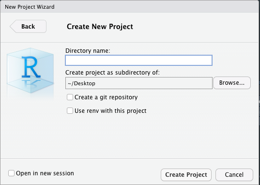
The first thing to do is to create a version-controlled directory. Version-controlled directories are called repositories, or repos for short. In RStudio, you can implement version control when you create a new RStudio project. Go to File > New Project > New Directory > New Project. You should see the following (by now familiar) window:

Ensure that the option Create a git repository is checked when creating your directory. You can give it whatever name you prefer: I named mine test_repo.

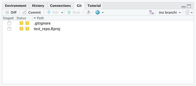
The newly created directory is your first Git repository; you can confirm this by double-checking that RStudio now shows a “Git” tab (by default close to the “Environment” tab in the top-right pane):

4.9.4 The basic lingo: “add” and “commit”

Git can have an overwhelming amount of jargon (you already encountered “repo”), but most of the time, you will be repeating the same two operations: adding and committing.

The point of Git is to save different versions of a file permanently. Permanently saving a new version is called committing. Once you have committed a new version of a file, it gets added to the file’s history; you can then look at it and go back to an older version.

While editing your file, you make many small changes but usually don’t want to save each as a new committed version permanently. Therefore, Git has a “staging area” (also called the index) where changes to a file are stored before being saved as a committed version. This is useful because sometimes you may want to:

• complete many small changes separately but save them all together as one new version.
• save changes as a backup in the short-term but do not want to save those changes in the long-term permanently.
• compare your current version with the last committed version without causing any conflicts in your repo.

In summary, when you make changes, you first add them to the staging area (also known as staging the changes). After making enough changes, you commit them, emptying the staging area and appending the new version to your repo’s version-control history.

4.9.5 Adding and committing in RStudio

The repository we just created is currently empty, so let us create a new R script called plot.R with the following code:

# Load packages
# Suite of packages for data manipulation and visualization
library(tidyverse)

# Load data from our GitHub
dat <- read.csv("https://raw.githubusercontent.com/EDUCE-UBC/educer/main/data-raw/data_intro_ws.csv")

# Create plot of oxygen by depth
quickplot(data = dat,
          x = O2_uM, 
          y = Depth_m)

Save this script in your RStudio project.

Now, look again at the RStudio Git pane. You will see that it contains three files: .gitignore, plot.R, and test_repo.Rproj. These are the three files located inside your RStudio project, as you can see in the RStudio Files pane, or simply by opening the folder in your computer (depending on your computer settings, the .gitignore file may be hidden).

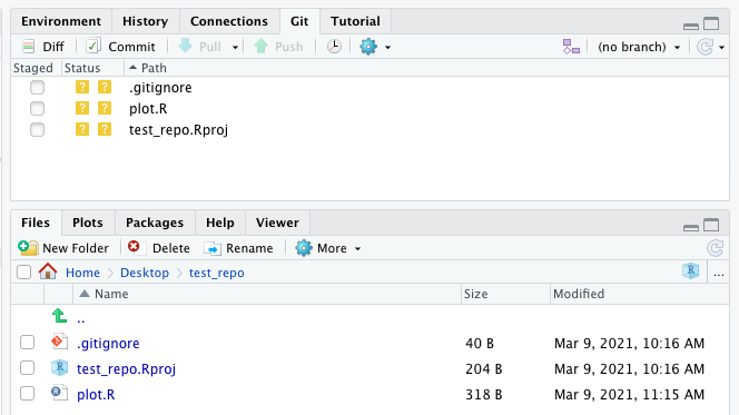
All three files are marked with yellow question marks indicating that they are “untracked,” i.e. Git is not yet keeping track of any changes to these files. We have to explicitly tell Git which files to track by adding them to the staging area.

To start tracking changes to these files, tick each file’s “Staged” box, adding them to the staging area. Notice how the files’ status changes from a question mark to a green capital A (which stands for “added”).

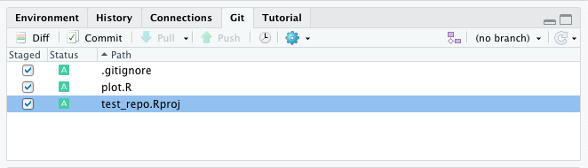
Now that we have added these files to the staging area, Git is ready to commit the current version into the version-control history.

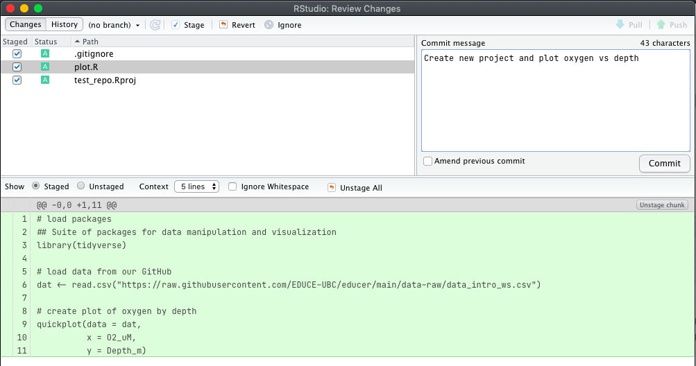
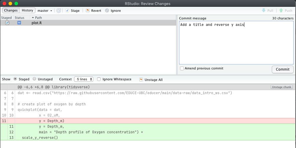
To store the current version of our project in Git’s history, click the “Commit” button taking us to the “Review Changes” window, where we can double-check the changes we made. At this point, we must write a commit message. The commit message is the name we give to the current project version. It should be short and descriptive, briefly explaining the changes we made. Later, when we look at our project’s history, you will identify different versions by their commit messages. Once the message is written, we can confirm the commit action by clicking the Commit button.

Note that the staging area is now empty (there are no files in the RStudio Git pane).

Let’s modify the plot.R script and save it:

# Load packages
# Suite of packages for data manipulation and visualization
library(tidyverse)

# Load data from our GitHub
dat <- read.csv("https://raw.githubusercontent.com/EDUCE-UBC/educer/main/data-raw/data_intro_ws.csv")

# Create plot of oxygen by depth
quickplot(data = dat,
          x = O2_uM, 
          y = Depth_m,
          main = "Depth profile of Oxygen concentration") +
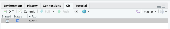
  scale_y_reverse()

Git detects that a tracked file has been modified and shows it with the blue capital M (which stands for “modified”). Tick the box to stage (add) the modifications we made.

Whenever you want to commit the modifications in the staging area, click the Commit button. The “Review Changes” window depicts the changes: deletions are red, and additions are green.

4.9.6 Viewing the commit history

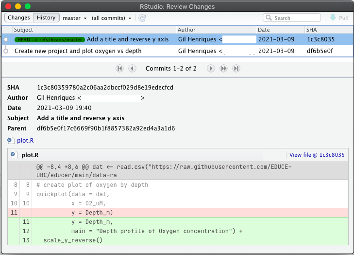
When you commit a new version, it gets added to the project’s version control history. You can display the history by clicking the clock button in the RStudio Git pane. The history window displays your project timeline, with the author, date and identifier of each commit, and the details of each commit changes in the lower part of the window:

4.9.7 Ignoring files

Generally speaking, you should track all the necessary files to reproduce your analysis. However, sometimes files are produced that we do not want to track, for example, temporary files.

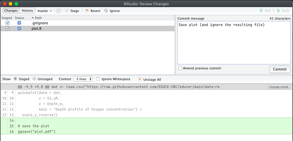
Let’s say we use our script to generate a figure, but we do not want to track changes to the figure. Add the command to save the plot to your script:

# Load packages
# Suite of packages for data manipulation and visualization
library(tidyverse)

# Load data from our GitHub
dat <- read.csv("https://raw.githubusercontent.com/EDUCE-UBC/educer/main/data-raw/data_intro_ws.csv")

# Create plot of oxygen by depth
quickplot(data = dat,
          x = O2_uM,
          y = Depth_m,
          main = "Depth profile of Oxygen concentration") +
  scale_y_reverse()

# Save the plot
ggsave("plot.pdf")

After saving and running the script, a new file (plot.pdf) will appear in your directory. Git will detect both the modified file and the new, untracked file:

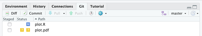
We do not want to track changes in the new plot.pdf file. One way of dealing with this situation is to simply never stage this file. If we do not stage it, it will remain untracked forever. However, this is quite annoying since the file will perpetually take up space in the RStudio Git pane.

Alternatively, we can tell Git explicitly not to track this file. To do so, right-click the file in the RStudio Git pane and choose “ignore”:

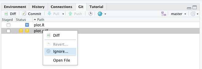
The effect of this, behind the scenes, is to add the name plot.pdf to the .gitignore file:

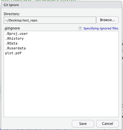
(An alternative way to do this is to manually open .gitignore and add plot.pdf to it.)

Once we ignore plot.pdf, it will no longer appear in the Git tab. Notice, also, that .gitignore has been modified. Stage and commit the changes.

4.9.8 Create a branch

One of the best ways to avoid the need to undo anything in Git is to use branches. These are parallel versions of your repo that you can work on independently of the main version. The main version of the project (the only one we have so far) is called the “main” branch (or “master,” but that name is increasingly discouraged).

A branch is like a parallel universe: any changes you make on the branch will not impact the main version of your project, but changes will still be version-controlled as you go. Imagine that we want to test some ideas, but we are not sure we want to incorporate them in the final project. We can create a new branch to test those ideas without disturbing our main, clean branch.

Branches are handy to:

• test new features without breaking the current working code.
• collaborate in parallel.
• follow a risky idea that has the potential to break your working code.
• develop the same base code into 2+ other applications.

We can have as many branches of the same repository as we want. You can then choose to merge the branch with main if you want to keep those changes or abandon the branch and go back to main if you do not want to keep those changes.

Let’s create a new branch. Click on the pink button close to the top-right corner of the RStudio Git pane (called the branch selector) to create a new branch called new_idea:

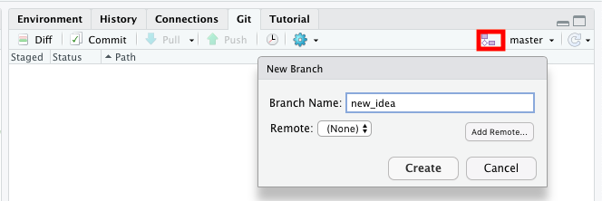
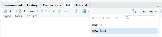
You have now created a new branch. You can switch between the main and the new_idea branches using the drop-down menu to the right of the branch selector. Make sure you are located on the new_idea branch.

Let’s create and save a new file, called boxplot.R:

# Load packages
# Suite of packages for data manipulation and visualization
library(tidyverse)

# Load data from our GitHub
dat <- read.csv("https://raw.githubusercontent.com/EDUCE-UBC/educer/main/data-raw/data_intro_ws.csv")

# Create plot of oxygen by depth
quickplot(data = dat,
          x = Season,
          y = O2_uM,
          geom = "boxplot")

Stage the new file and commit it with an appropriate commit message. Then, open the repository history by clicking the clock button.

Notice how the new_idea repository (which has a big green label called “HEAD”) is up-to-date, containing the most recent commits. In contrast, the main branch is one step behind:

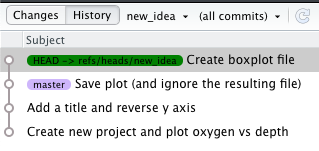
The HEAD is the commit you are currently viewing. In our case, the HEAD points to the most recent commit in the current branch. The HEAD label is transferred to the other branch when you switch branches.

Let’s imagine that we now want to improve some code on our main branch. Having several branches allows us to work independently on one without disturbing the other. Switch back to the main branch using RStudio’s branch selector. If RStudio asks you whether you want to close boxplot.R because “it has been deleted or moved,” click Yes.

Now that you switched to the main branch look at your project directory. You can do this by opening the project folder on your computer or by looking at the contents of the “Files” tab in RStudio. You will see that the folder contains the following files: plot.pdf, plot.R, and test_repo.Rproj (besides hidden files such as .gitignore). What happened to the file boxplot.R? Does it no longer exist?

In fact, the file boxplot.R still exists, but it exists only when HEAD is pointing to the new_idea branch. It is like you are hopping between parallel versions of your project: the new_idea branch contains this file, but not the main branch. You can try switching back and forth between the branches to see the file boxplot.R appear and disappear from your directory.

Now let’s make some changes to the plot.R file. Make sure you are in the main branch and change the plot so that the points are colored by the Season:

# Load packages
# Suite of packages for data manipulation and visualization
library(tidyverse)

# Load data from our GitHub
dat <- read.csv("https://raw.githubusercontent.com/EDUCE-UBC/educer/main/data-raw/data_intro_ws.csv")

# Create plot of oxygen by depth
quickplot(data = dat,
          x = O2_uM,
          y = Depth_m,
          color = Season,
          main = "Depth profile of Oxygen concentration") +
  scale_y_reverse()

# Save the plot
ggsave("plot.pdf")

Save the script, then stage and commit your changes with an appropriate commit message.

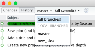
View your repository history again, clicking on the clock button. In the drop-down menu on the top-left corner of the history window (which says main), select the option “(all branches).”

Notice the branching structure in your history:

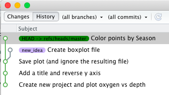
The HEAD label has moved to the current branch. Note that each branch has changes that the other branch doesn’t have. The new_idea branch has the boxplot file. The main branch has points colored by season.

4.9.9 Merging two branches

At this point, you could work more on the main branch or decide to switch back to new_idea and improve the code there. But let’s imagine that you are happy with the code in the new_idea branch and want to incorporate it into your main branch. This is called merging the new_idea branch into the main branch.

Unfortunately, there is no easy way to do this using the RStudio graphical interface. To merge, we will need to use the terminal. First, make sure you are in the main branch. Then open the terminal and navigate to your project’s directory. Finally, type:

git merge new_idea -m "Incorporate code for boxplot"

Git terminal commands always start with the keyword git, followed by the action we want to perform: merge. Then, we state the branch that we want to merge: new_idea. Finally, we provide a short description after the -m flag.

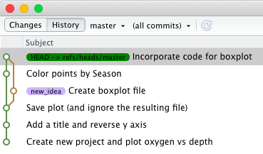
After merging, the main branch will contain all the originally made changes in the new_idea branch. In particular, the file boxplot.R should now be present in the main branch. Verify this by opening the project folder or checking its contents in the RStudio Files tab. At this point, you could keep committing your work to the main branch until the next time you feel the need to create a branch.

You can also take a look at the “History” window to see the full branching history so far:

4.9.10 Merge conflicts

Merging works simply if

• only one of the branches has been altered since their branch point.
• the changes occurred in different files (as was the case in our example above).
• or even if the changes occurred in different regions of the same file.

But what if both branches contain changes to the same line of text (non-synonymous changes)? Then, there will be a conflict.

Create a new branch named color_by_depth. In the new branch, change the file plot.R from color = Season to color = Depth_m, resulting in a plot where points are colored by depth (using a continuous color scale) instead of season. Commit this change with an appropriate commit message.

Now, return to the main branch. In the main branch, change color = Season to color = O2_uM. The points are now colored by oxygen concentration. Commit this change.

These two changes are clearly incompatible. So what happens when we merge the two branches? Making sure you are in the main branch, use the terminal to merge color_by_depth.

Look at the message that appears in the terminal: an all-caps CONFLICT, warning that Automatic merge failed, with instructions to fix conflicts and then commit the result.

Back in RStudio, the Git pane indicates the status of plot.R with a yellow capital U, which stands for “unmerged.” We need to resolve the merge conflicts. Look at the script of the file plot.R. The markers <<<<<< HEAD and >>>>>> color_by_depth surround the region containing conflicted code. The two versions (HEAD and color_by_depth) are separated by the marker =======:

quickplot(data = dat,
          x = O2_uM,
          y = Depth_m,
<<<<<<< HEAD
          color = O2_uM,
=======
          color = Depth_m,
>>>>>>> color_by_depth
          main = "Depth profile of Oxygen concentration") +
  scale_y_reverse()

Simply edit the code manually until you have the version you want to resolve the conflict. Save the file and commit the new, corrected version. Conflict solved!

4.9.11 Time travelling!

RStudio’s interface provides a “Revert” action (click on the blue gear button in the Git pane) to revert the project to the last recorded state in the repository. However, sometimes you want to revert to an older state of the repository. RStudio does not offer a button for this, so we have to use the terminal and enter commands manually.

Let’s say that after all of these changes to the color of the points, we decide we aren’t actually pleased and prefer to go back to when the points were colored by season. Let’s look at the Git history to get the SHA identifier of the commit we want to revert to. In the image below, that corresponds to the SHA identifier 56b6a147 (highlighted in red below), but your identifier will be different:

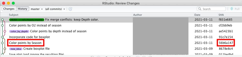
Open the terminal, navigate to the project directory, and type the command to revert to your SHA identifier (in the example above, it would be commit 56b6a147):

git checkout <SHA ID>

We get a somewhat scary message:

Note: checking out '<SHA ID>'.

You are in 'detached HEAD' state. You can look around, make experimental
changes and commit them, and you can discard any commits you make in this
state without impacting any branches by performing another checkout.

If you want to create a new branch to retain commits you create, you may
do so (now or later) by using -b with the checkout command again. Example:

  git checkout -b <new-branch-name>

HEAD is now at <SHA ID>... Color points by Season

What does “'detached HEAD' state” mean? Before, your learned that HEAD is simply a label for the current, active branch. But the HEAD label identifies not only the active branch but the active version of that branch.

Before using the checkout command, the HEAD was on the most recent commit of the main branch. But now, the HEAD is no longer on the tip of the branch. It is on an older version: this is what “detached HEAD” means.

The terminal message informs us, quite helpfully, that “HEAD is now at <SHA ID>... Color points by Season”. This is precisely what we wanted. We travelled back to when the points were colored by season, so that is now the active version of the project (i.e., it is now the HEAD).

The History window may help make this clear:

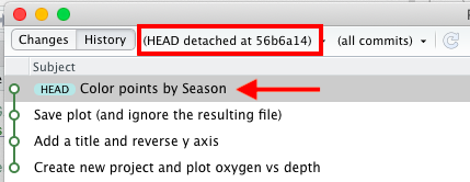
If you look at the plot.R script, you will see that we are back to the older version of the plot.

At this point, there are two possibilities:

1. If we would like to start working again from this time point, we could make a new branch stem from this point using RStudio, just like we did before.

2. Alternatively, we could return to the tip of the main branch by using the branch selector in RStudio and selecting that branch.

For this workshop, let’s return to the main branch. If you prefer, you can also create a new branch, just for practice, but if you do so, return to the main branch afterward to follow along with the workshop.

You should now be on the main branch with points of the plot colored by depth.

Often, we want to revert just one file to an older state, not the entire project. For instance, let’s say we want to go back to a very old version of our plot right after we reversed the y-axis. Let’s find the identifier in the project History:

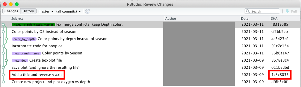
The problem is this version of the plot is so old that it predates the creation of the boxplot.R file. We want to revert our plot.R code to this older version (the SHA identifier is 1c3c8035 in the image above), but we don’t want to lose or change all the other files in our project. Fortunately, we can time-travel a single file like this (again, you will need to use your own appropriate identifier):

git checkout <SHA ID> -- plot.R

We didn’t get a “detached HEAD” warning this time because, instead of going back to a previous time point along the branch, Git replaced the current version of a file (plot.R) with its previous version. You can see that the script plot.R in RStudio has now reverted to the old version. The RStudio Git pane lists the file as modified because the older version (to which it has been restored) is different from the previously-existing version.

At this point, you can either:

1. stage and commit the “modified” version of plot.R (which is just an older version).

2. decide to discard this restored version and revert to the latest recorded version by clicking the gear button and selecting the “Revert” action.

4.10 Introduction to GitHub

GitHub is a web service for hosting Git repositories. It has web and GUI interfaces as well as many tools for collaborating on repos.

Similar to our decision to use Git, GitHub’s strengths are its popularity and ease of use. If you choose Git, GitHub is the natural choice for hosting your projects online and collaborating with others.

Before this workshop, you should have signed up for a free GitHub account (check the setup instructions here). As part of the setup, you need to link your computer to your GitHub account using the email from this account and whatever name you want stamped on your commits. This need only be done once on your computer.

git config --global user.name "<your GitHub username>"

git config --global user.email "<your GitHub account email>"

There are two main uses of GitHub. One is backing up your work in the cloud with the option to share it with other researchers. The second is for online collaboration. We will start with the first.

4.10.1 GitHub for online version control

One advantage of using GitHub is that it keeps a copy of your repositories in the cloud. An online copy of a repository, hosted on GitHub, is called a remote repo. If you lose your computer, all your code will still be available on the remote. Furthermore, you can use GitHub to work on a repo from multiple computers since you can sync any changes you do with the remote. Finally, you can share your work with other people, since (if you make your remote repos public) they can download the project onto their computers.

After creating an online repo, you can sync it with your local repository. You can then make changes (on your computer) to the local version of the repository, using the add-commit framework that you learned before. Once you have done changes, you need to upload those changes to the remote version of the repository: in Git jargon, you need to “push” the changes to the remote.

4.10.1.1 Make an online repo (remote repo)

Let’s get started by making an online GitHub repo. Our ultimate goal is to get our test_repo repository on GitHub, but we need to start by creating a blank remote repo on GitHub.

Navigate to your GitHub account homepage in a browser. On the left-hand side of the page, find the Repositories section and click the green button labelled New.

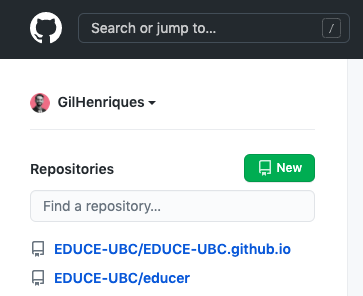
Name the repo test_repo and create it. GitHub then gives you the URL for this repo.

4.10.1.2 Link local and online repo

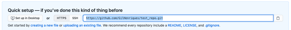
We will sync our local test_repo to the online GitHub (remote) repo using the URL provided.

Using your terminal, navigate to the test_repo directory. Then, enter the following code (using your specific repo URL). You can also copy this code from the GitHub page, which is currently open.

git remote add origin <remote repo URL>
git branch -M main
git push -u origin main

If no errors occur, you can go back to your browser and refresh your page. You should now see all the files in your online repo.

Once your local repo is fully linked with its online GitHub repo, you can use Git as you normally would (change files, add, and commit). Let’s make a change in our plot.R file. We will map the shape of the points in our plot to the column Season:

# Create plot of oxygen by depth
quickplot(data = dat,
          x = O2_uM,
          y = Depth_m,
          color = Depth_m,
          shape = Season,
          main = "Depth profile of Oxygen concentration") +
  scale_y_reverse()

Save the changes, add and commit (with an appropriate commit message). We can now upload the changes we just committed onto the remote on GitHub by clicking on the green upward arrow labelled “Push”:

4.10.1.3 Multiple computers

If you are the only one working on your repo and only from one computer, GitHub acts as a one-way street. You push things there for storage, sharing, etc. and should only need to pull them back down if something terrible happens to your computer.

However, since this repository has an online copy, GitHub allows you to work on the same repo from multiple computers. All you need to do is ensure that all computers are in sync with each other and with the remote.

4.10.1.3.1 Clone an online repo

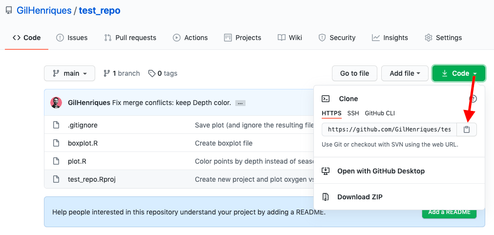
Let’s say you create test_repo using computer A. You pushed it onto GitHub, creating a remote copy of test_repo. Now, when you go to computer B, you need to start by copying the remote repo to computer B. Copying a (remote) repo from GitHub into a (local) computer is called “cloning” the repo.

RStudio makes cloning easy. On computer B, open the GitHub repository page (you can follow along on your computer for this workshop). Click the green drop-down button labelled “Code,” and copy the URL:

You have now copied the URL of the repository. Now, open RStudio. Recall, at this point in your workflow, you are working from computer B, where you don’t have any test_repo project. So you need to create this project using the standard RStudio method (go to File > New Project). But at this point, instead of the usual option (File > New Project > New Directory), you chose the option File > New Project > Version Control:

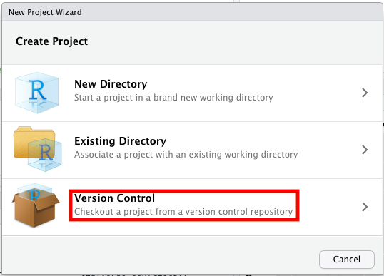
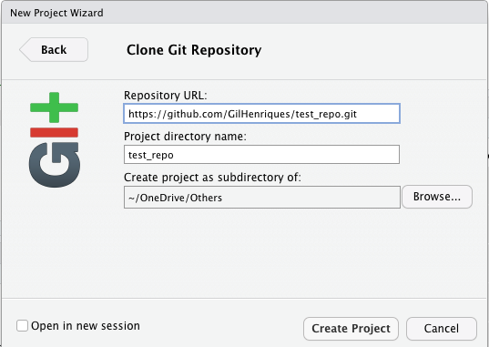
Select the option Git and, under “Repository URL,” paste the URL you copied from GitHub. Under “Repository name”, write test_repo. Chose where, on your computer, you want to create this local directory.

You have now cloned (downloaded a copy of) test_repo on computer B! You can now make and commit changes to the repository on that computer and push them to the remote repo when you are satisfied.

4.10.1.3.2 Pull changes from the online repo

Now when you have multiple copies of a repo potentially being worked on and pushed to GitHub from various computers, the version on GitHub may be more up-to-date than the one you have on the computer you happen to be working on currently. For instance, if you make changes on computer B and push them to GitHub, the repo on GitHub will be more up-to-date than on computer A. When you return to computer A, you need to download the changes from GitHub into computer A.

You can think about this as the reverse of pushing changes to GitHub. For that reason, this is called “pulling” changes from the remote repo into the local repo. All you have to do is click on the blue downward arrow labelled “Pull”:

Once you do so, all the changes will be downloaded from GitHub into your local computer, and you will be up-to-date.

4.10.2 GitHub for collaboration

Since you now know how you can work on the same repo from multiple computers, you can see how a similar setup enables collaborators to work on the same project.

Let’s say you are working closely together with a collaborator. The owner of the remote repository needs to add the other person as a collaborator on GitHub. Then, both you and your collaborator can pull and push changes to the same project.

To add a collaborator to your GitHub repo, go to its page > Settings > Manage access > Invite a collaborator. Once your collaborator accepts the invitation, they will be able to clone the remote repository onto their computer. Both of you can collaborate on the same project from that point on. Remember to always hit Pull before starting to work to ensure that you have the most up-to-date version of the project!

---

End of workshop

---

4.11 Additional resources

4.11.1 Reproducible research

• Software Carpentry including lessons on Git, Rmd, and reproducible research
• Riffomonas including reproducible research methods in R

4.11.2 R/RStudio

• renv tutorial
• R Markdown cheatsheet
• R Markdown tutorials
• Git in RStudio

4.11.3 Git/GitHub

• Git cheatsheet
• List of all Git commands
• Git tutorial
• Pro Git Book
• GitHub help
• Build a web site from a repo!
• Explore GitHub Education benefits for students and teachers

4.12 Survey

Please provide us with feedback through this short survey.