8 HTSeq and DESeq2
8.1 Overview
In this tutorial, we will use DESeq2 to analyze some RNA-Seq data. This tutorial covers how to:
Use HTSeq on data you generated on your own.
Load counts from new data (not your own) into R.
Set controls for DESeq2 by changing factor levels.
Run sanity checks to ensure your results make biological sense.
Filter differential expression tables by Padj and Log2 fold change.
8.2 HTSeq Overview
Normally, you would use HTSeq to create your count files from the STAR alignments you produced, using the following code:
pip3 install htseq

htseq-count \
  <sample_id>/<sample_id>.fastq.gzAligned.sortedByCoord.out.bam \
  Mus_musculus.GRCm38.84.gtf \
  -f bam \
  -r pos \
  --stranded=no \
  > <sample_id>.htseq.out
…and repeat for every sample.
However, due to constraints on time and available disk space on the server, we will be downloading existing count data from an experiment containing six samples grouped into control and treatment categories.
8.3 DESeq2
8.3.1 Setup
All of the data for this tutorial is located on the Orca1 server in /projects/micb405/resources/DESeq2_tutorial. Use scp to copy the entire directory to your computer and move the directory to where you keep your MICB405 files.
Open RStudio and create a new R project (File > New Project).
Since we want all of our DESeq2 tutorial materials together, click on ‘Existing Directory’ and choose the DESeq2_tutorial directory that you copied from the server.
8.3.2 Scripting in R
One of the most critical aspects of bioinformatics is ensuring that your code is easy to read and well documented. This means that you should organize scripts and use comments to split your code into different sections.
8.3.2.1 Setting up your script
You should always begin an R script with a simple header:
# Your name
# Title of your script (e.g. MICB405 DESeq2 tutorial)
# Date of your last update
The next step of any R script is to load all of the packages that you plan to use:
Be sure to install any packages you have not installed previously on your laptop.
DESeq2 will need to be downloaded with BiocManager:
8.3.2.2 Loading data
It is best practice to collect all input files in a folder (most often called “data”) from which files will only be loaded but not overwritten.
Since there are multiple input files, we can use R to generate paths to the files we want to open automatically. All of the data files are in the same directory, so to save us some typing, we can assign the path to that directory as a variable.
dir <- "data"Each filename is generated from the sample name and a common suffix. To get a vector of sample names, we can use the samples.csv metadata file, which we will also need to assign conditions to samples. When you work on your projects, you will enter the filenames and the corresponding conditions yourself into a CSV file.
#  file.path constructs filepath with the correct separator dependent of OS
sample_metadata <- read_csv(file.path(dir, "samples.csv"))
sample_metadata
## # A tibble: 6 × 2
## sample condition
## <chr> <chr>
## 1 control_1 control
## 2 control_2 control
## 3 control_3 control
## 4 treat_1 treatment
## 5 treat_2 treatment
## 6 treat_3 treatmentAs you can see, the metadata has two columns: sample names and conditions. We can generate filenames from sample_metadata$sample for each element in the vector (e.g. the first element is "control_1") by adding the directory "data" as prefix and ".htseq.out" as suffix.
#  paste0 appends (i.e. adds together) character objects
files <- paste0(file.path(dir, sample_metadata$sample), ".htseq.out")
files
## [1] "data/control_1.htseq.out" "data/control_2.htseq.out"
## [3] "data/control_3.htseq.out" "data/treat_1.htseq.out"
## [5] "data/treat_2.htseq.out" "data/treat_3.htseq.out"Then, as a quick test, you can run all(file.exists(files)), which should return TRUE to your console if the file paths are correct. First, files.exists(files) checks for each filename in files if that file exists and returns TRUE or FALSE, resulting in a logical vector. If all files are present, then all elements in the logical vector will be TRUE.
file.exists(files)## [1] TRUE TRUE TRUE TRUE TRUE TRUEThe function all() only returns TRUE if all elements of a logical vector are TRUE.
all(file.exists(files))## [1] TRUE8.3.3 Running DESeq2
DESeq2 requires that all of your data be in the shape of a SummarizedExperiment object. Since reshaping your input data with your code would be complicated, there are functions within DESeq2 specific for the source of your counts file, which will prepare your data for use in DESeq2. Since we are using HTSeq to generate our counts data in this class, the function we need is called DESeqDataSetFromHTSeqCount(). One of the required arguments is sampleTable, which must provide a data table with columns for sampleName, fileName, and any of the independent variables you changed in your experiment (e.g. sex, treatment, tissue). For that purpose, we can quickly build sample_df from the loaded metadata sample_metadata and the vector of file paths files that we defined earlier.
The other required argument for DESeqDataSetFromHTSeqCount() is design. The design argument is a formula designated by the tilde symbol ~ and identifies which independent variable(s) you want to investigate. In our data, we have only a single independent variable, i.e. condition. Experiments with multifactorial experimental design are a lot more complicated to investigate.
# Creates a new data table with the variables sampleName, fileName and condition
sample_df <- data.frame(sampleName = sample_metadata$sample,
                        fileName = files,
                        condition = sample_metadata$condition)

ddsHTSeq <- DESeqDataSetFromHTSeqCount(sampleTable = sample_df,
                                       design = ~ condition)
In a DESeq data set, the design variables are stored as a factor (a data type in R), which by default are organized alphabetically. Without further information, DESeq2 will use the condition that comes first alphabetically as reference. If you were using "treated" and "untreated", for example, DESeq2 would incorrectly assume that the "treated" samples are the reference. To prevent any confusion, we can set the name used as reference explicitly with the argument ref inside the relevel() function.
## Set control condition using the relevel function
ddsHTSeq$condition <- relevel(ddsHTSeq$condition, ref = "control")
Now that the reference level has been set, we can run DESeq2 on the dataset.
dds <- DESeq(ddsHTSeq)8.3.4 Sample Clustering
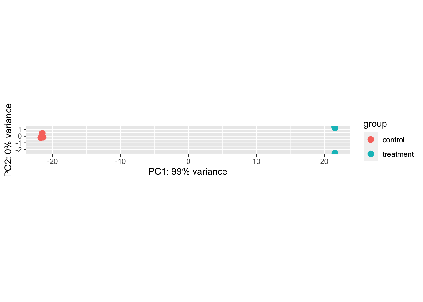
Because the distribution of RNA Seq data is highly skewed, with a few high abundance genes and many low abundance genes, it is helpful to transform our data to visualize clustering. DESeq2 comes with the function rlog(), which log-transforms your count data. After transformation, we can use PCA to identify which samples are more similar and if they group by one or more of the independent variables (in our case, we have only a single variable that can take “control” or “treated”).

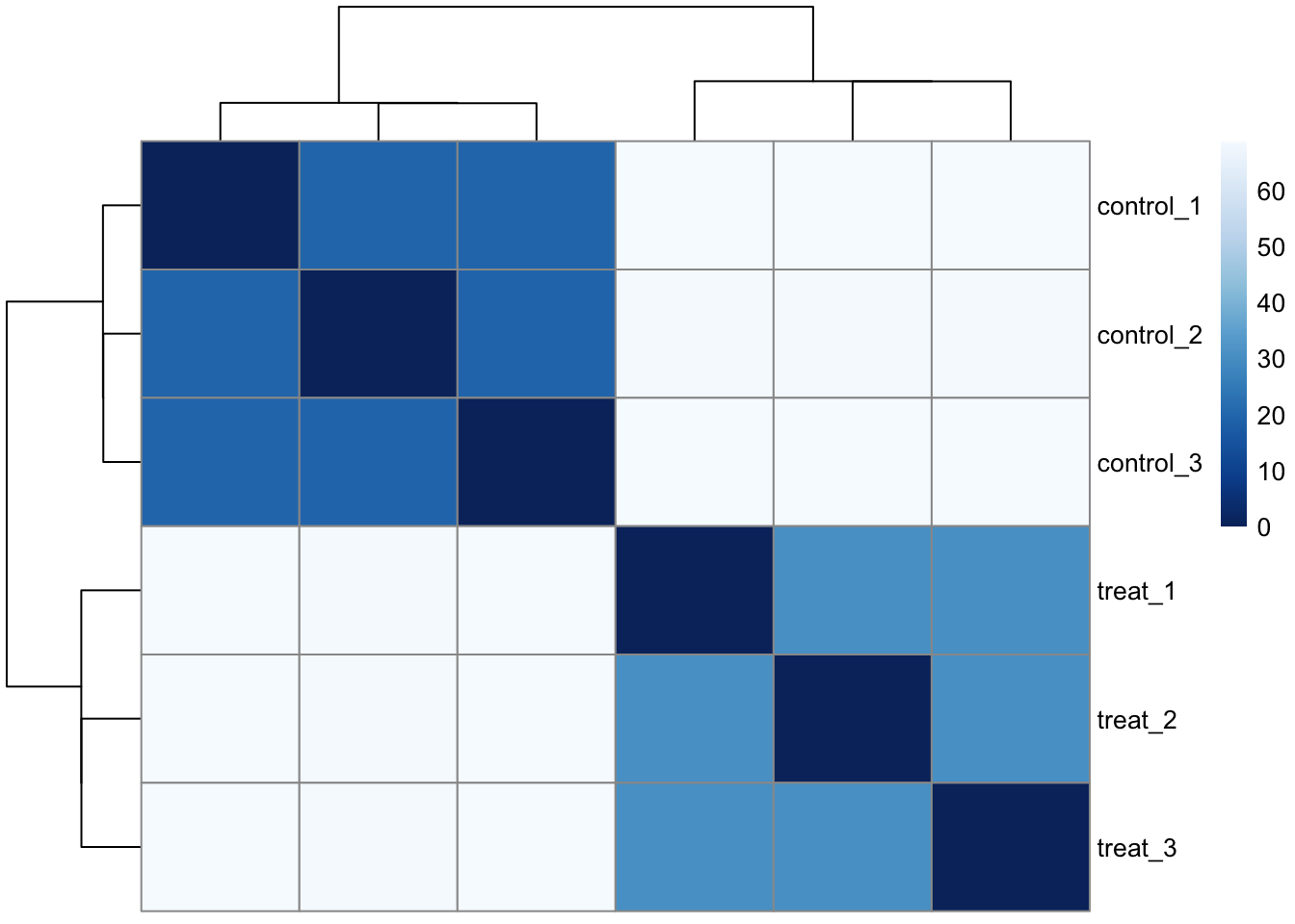
A distance matrix is another way to examine how samples cluster. The code chunk below calculates distances between each sample and then maps a colour palette (defined with colorRampPalette) onto it so that more similar samples display darker colours.
sample_dists <- dist(t(assay(rld)))
sample_dist_matrix <- as.matrix(sample_dists)
colnames(sample_dist_matrix) <- NULL
colours <- colorRampPalette(rev(brewer.pal(9, "Blues")))(255)
pheatmap(sample_dist_matrix,
         clustering_distance_rows = sample_dists,
         clustering_distance_cols = sample_dists,
         col = colours)
If the samples don’t cluster together like you would expect them to, check for batch effects.
8.3.5 Filtering and data export
Since our samples cluster according to the independent variable, we can move forward with our analysis. To examine our results, we can save them to our global environment. DESeq2 calculates results for all combinations of levels in your experimental design. The resultsNames() function tells us the name of each result that DESeq2 has calculated, so we can choose which one to look at by specifying “name =” in results(). The results() function will output a matrix of all genes, including those with similar or differential expression between the two conditions.
resultsNames(dds)## [1] "Intercept" "condition_treatment_vs_control"## log2 fold change (MLE): condition treatment vs control
## Wald test p-value: condition treatment vs control
## DataFrame with 6 rows and 6 columns
## baseMean log2FoldChange lfcSE stat pvalue
## <numeric> <numeric> <numeric> <numeric> <numeric>
## ENSMUSG00000000001 299.611431 -1.15529 0.0952683 -12.126645 7.63122e-34
## ENSMUSG00000000003 0.217348 1.75589 4.0804729 0.430316 6.66966e-01
## ENSMUSG00000000028 10.401452 1.75564 0.5135561 3.418600 6.29442e-04
## ENSMUSG00000000031 0.000000 NA NA NA NA
## ENSMUSG00000000037 2.760919 2.66847 1.1572396 2.305895 2.11165e-02
## ENSMUSG00000000049 0.900647 1.37848 2.6339604 0.523348 6.00732e-01
## padj
## <numeric>
## ENSMUSG00000000001 3.52493e-32
## ENSMUSG00000000003 NA
## ENSMUSG00000000028 3.32121e-03
## ENSMUSG00000000031 NA
## ENSMUSG00000000037 6.23462e-02
## ENSMUSG00000000049 NASince we are only interested in differentially expressed genes, we can use the subset() function from base R to keep results with an adjusted p-value < 0.05 and then save the results to a CSV file.
significant_res <- subset(res, padj < 0.05)
write.csv(as.data.frame(significant_res), file = "treat_vs_control_05.csv")
If you want more information about DESeq2, you can access the package vignette by running:
vignette("DESeq2")Now that you have a distance matrix and a list of significant genes, what is one downstream analysis you could do that could inform you about a biological difference between the two treatment groups?
8.4 Additional resources
Original paper: An RNA-Seq atlas of gene expression in mouse and rat normal tissues