A The Saanich Inlet data set

A.1 Description

We will work with real-world data collected as part of an ongoing oceanographic time series program in Saanich Inlet, a seasonally anoxic fjord on the East coast of Vancouver Island, British Columbia:

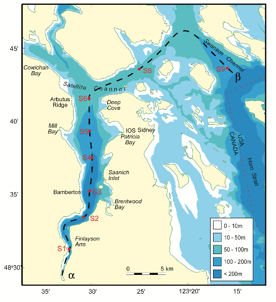
FIGURE A.1: The Saanich Inlet

Figure A.1 shows a map of Saanich Inlet indicating conventional sample collection stations (S1-S9). The data used in this tutorial (sourced from S3, Cruise 72) include various geochemical measurements and the genomic and transcriptomic data of microbial samples at depths 10, 100, 120, 135, 150, 165 and 200 m.

For more details about these data, see (14), and for more detailed information on the environmental context and time series data, see (15).

A.2 Data on the server

The Saanich data is located on the MICB425 server at /mnt/datasets/saanich/.

/mnt/datasets/saanich/
├── [   0]  directory_structure.txt
├── [492M]  MAGs
│   └── [492M]  Concatenated
│       └── [492M]  All_SI072_Metawrap_MAGs.fa
├── [3.5G]  MetaG_Assemblies
│   ├── [630M]  SI072_100m_contig.fa
│   ├── [525M]  SI072_10m_contig.fa
│   ├── [571M]  SI072_120m_contig.fa
│   ├── [505M]  SI072_135m_contig.fa
│   ├── [396M]  SI072_150m_contig.fa
│   ├── [748M]  SI072_165m_contig.fa
│   └── [219M]  SI072_200m_contig.fa
│   └── [3.5G]  SI072_All_contigs.fa
├── [ 64G]  MetaG_Trim_QC_Reads
│   ├── [4.7G]  SI072_100m_pe.1.fq.gz
│   ├── [4.7G]  SI072_100m_pe.2.fq.gz
│   ├── [4.2G]  SI072_10m_pe.1.fq.gz
│   ├── [4.2G]  SI072_10m_pe.2.fq.gz
│   ├── [4.2G]  SI072_120m_pe.1.fq.gz
│   ├── [4.2G]  SI072_120m_pe.2.fq.gz
│   ├── [4.4G]  SI072_135m_pe.1.fq.gz
│   ├── [4.4G]  SI072_135m_pe.2.fq.gz
│   ├── [4.8G]  SI072_150m_pe.1.fq.gz
│   ├── [4.7G]  SI072_150m_pe.2.fq.gz
│   ├── [6.5G]  SI072_165m_pe.1.fq.gz
│   ├── [6.4G]  SI072_165m_pe.2.fq.gz
│   ├── [3.3G]  SI072_200m_pe.1.fq.gz
│   └── [3.3G]  SI072_200m_pe.2.fq.gz
├── [ 54G]  MetaT_Raw_Reads
│   ├── [8.9G]  SI072_100m_MetaT_QC_Filtered.fastq.gz
│   ├── [6.4G]  SI072_10m_MetaT_QC_Filtered.fastq.gz
│   ├── [6.8G]  SI072_120m_MetaT_QC_Filtered.fastq.gz
│   ├── [7.2G]  SI072_135m_MetaT_QC_Filtered.fastq.gz
│   ├── [10.0G]  SI072_150m_MetaT_QC_Filtered.fastq.gz
│   ├── [8.7G]  SI072_165m_MetaT_QC_Filtered.fastq.gz
│   └── [6.0G]  SI072_200m_MetaT_QC_Filtered.fastq.gz
├── [181M]  SAGs
│   └── [181M]  Concatenated_Med_Plus
│       └── [181M]  Saanich_Med_Plus_SAGs.fasta
└── [ 42K]  seq2lineage_Tables
    ├── [ 17K]  Med_Plus_SAGs_GTDB_Taxonomies.tsv
    └── [ 25K]  SI072_MAGs_All_GTDB_taxonomies.tsv

 122G used in 8 directories, 33 files

Additionally, if you would like to run GTDB-TK, the path to the GTDB refrence directory is located at /mnt/datasets/GTDB-Tk/release95/

A.3 Description of input data

List of directories and their contents

• MAGs

  Within the Concatonated subdirectory, there is a single All_SI072_Metawrap_MAGs.fa fasta file which you will use with both treesapp assign and treesapp update. After the MAGs were generated with the MetaWrap pipeline (16) (see Methods), sample IDs were added to the contig headers of each MAG produced from each SI072 sample depth. The individual MAGs were then concatenated into this file.

• MetaG_Assemblies

  This directory contains seven assembled metagenomic contigs for each SI072 sample depth, and one file where each of these has been concatonated into a single file. These files will be used for the treesapp assign and abundance tutorials. These files were generated by assembling the trimmed and quality controlled reads that were generated by the Illumina HiSeq platform (see Methods).

• MetaG_Trim_QC_Reads

  This directory contains fourteen fastq files which contain the paired-end forward and reverse metagenomic reads for each SI072 sample depth. These trimmed and QC’d fastqs were generated by processing the raw reads through the Megahit workflow described below. You will use these files for treesapp abundance to get the metagenomic abundance of your assigned genes.

• MetaT_Raw_Reads

  This directory contains seven filtered and QC’d metatranscriptome fastq files for each SI072 Sample depth. These files are paired end and interleaved. These files we provided by the the JGI and generated based on the methodology below. You will use these files in treesapp abundance to calculate the metatransciptomic abundances of each gene of interest.

• SAGs

  Within the Concatenated_Med_Plus subdirectory, there is a single Saanich_Med_Plus_SAGs.fasta file which you will use with both treesapp assign and treesapp update. After the MAGs were generated with the SAG Assembly and Decontamination Workflow (17–20) (see Methods), sample IDs were added to the contig headers of each MAG produced from each SI072 sample depth. The individual MAGs were then concatenated into this file.

• seq2lineage_Tables

  This directory contains two files that will be used for treesapp update. One file contains the lineage information from the MAGs, and the other contains information for the SAGs. These tables were generated by taking each separate MAG and SAG respectively and passing them through the Genome Taxonomic Database Toolkit v1.4.0 classify workflow (7) (see Methods). Then, the first two columns of the archaeal and bacterial summary files were taken and combined into each of these files.

A.4 Methods

A.4.1 Metagenomes and metatransriptopmes

A.4.1.1 Sample Collection

Water was collected at 10, 100, 120, 135, 150, 165, and 200m at Saanich Inlet on August 1st, 2012 and filtered through a 0.22 µm Sterivex filter to collect biomass. Total genomic DNA and RNA were extracted from these filters. RNA was reversed transcribed into cDNA and both genomic DNA and cDNA were used in the construction of shotgun Illumina libraries. Sequencing data were generated on the Illumina HiSeq platform with 2x150bp technology. For more in-depth sampling and sequencing methods, please see (21).

A.4.1.2 Quality filtering of reads

The resulting reads were processed, quality controlled and filtered with Trimmomatic (v.0.35, documentation) (17). Trimmomatic command is as follows, where SI072_XXX represents the same command being applied to each of the seven depths.

trimmomatic -threads 8 -phred33 \
Path_to/SI072_XXXm/Raw/forward_dir/SI072_XXXm_R1.fastq \
Path_To/SI072_200m/Raw/reverse_dir/SI072_XXXm_R2.fastq \

Path_To/SI072_200m//trim/SI072_XXXm_pe.1.fq \

Path_To/SI072_200m//trim/SI072_XXXm_pe.2.fq \

ILLUMINACLIP:/usr/local/share/Trimmomatic-0.35/adapters/TruSeq3-PE.fa:2:3:10 LEADING:3 TRAILING:3 SLIDINGWINDOW:4:15 MINLEN:36

The resulting trimmed fastq files were also deposited into the MICB425 server in /mnt/datasets/saanich/MetaG_Trim_QC_Reads

A.4.1.3 Contig Assembly

MEGAHIT (v.1.1.3, documentation) (22) was used to assemble the filtered metagenomic reads into contigs.

megahit -1 Path_To/SI072_200m//trim/SI072_XXXm_pe.1.fq  -2 Path_To/SI072_200m//trim/SI072_XXXm_pe.2.fq  -m 0.5  -t 12  -o megahit_result --k-min 27 --k-step 10 --min-contig-len 500

The resulting assemblies can be found in /mnt/datasets/saanich/MetaG_Assemblies.

A.4.1.4 Binning and MAG Generation

MetaWRAP (v1.2.4, documentation) (16) was used to generate the MAGs from the metagenome assemblies and filtered reads for this project. MetaWRAP leverages multiple binning software (we chose to use MetaBAT2 v2.12.1 (23) and MaxBin v2.2.7 (24), (25)) to create a non-redundant set of MAGs that are better quality than those from any single software. The quality of the resulting bins – assessed by their completeness, contamination, and strain-heterogeneity – was calculated with MetaWRAP’s implementation of CheckM (v1.0.12) (19). The command used to invoke MetaWRAP is as follows:

metawrap binning -a SI072_Assembly.fa -o output_directory -t 16 -m 64 -l 1500 --metabat2 --maxbin2 --universal Path_To/SI072_200m//trimSI072_XXXm_pe.1.fastq Path_To/SI072_200m//trimSI072_XXXm_pe.2.fastq

A.4.1.5 Taxonomic Assignment of MAGs

The resulting MAGs were then passed through GTDB-TK v1.4.0 classify workflow with the reference data version r95 documentation (7).

gtdbtk classify_wf --genome_dir Path_To_SI072/MAGs/ -x .fa --out_dir Path_To_SI072/MAG_GTDB_Outputs/ --cpus 8 --pplacer_cpus 8

After updating the headers for resulting 219 bins with the sample IDs, the bins were concatenated and deposited into: /mnt/datasets/saanich/MAGs/Concatenated/

A.4.2 Single-Cell Amplified Genomes

A.4.2.1 Sample Collection

Water was collected at across the water column at Saanich Inlet on August 9th, 2011. 900 µL of seawater was aliquoted into 100 µL of glycerol-TE buffer, then stored at -80 degrees Celsius. Samples from 100m, 150m, and 185m were selected for sorting and sequencing. The selected samples were thawed and had their microbial cells sorted at the Bigelow Laboratory for Ocean Sciences’ Single Cell Genomics Center (scgc.bigelow.org).

A.4.2.2 Florescence Activated Cell Sorting

Samples were passed through a sterile 40 𝜇m size mesh before microorganisms were sorted by a non-targeted isolation procedure. For non-target isolation, the microbial particles were labeled with a 5 𝜇M final concentration of the DNA stain SYTO-9 (Thermo Fisher Scientific). Microbial cells were individually sorted using a MoFloTM (Beckman Coulter) or an InFluxTM (BD Biosciences) flow cytometer system equipped with a 488 nm laser for excitation and a 70 μm nozzle orifice30. The gates for the untargeted isolation of microbial cells stained with SYTO-9 were defined based on the green fluorescence of particles as a proxy for nucleic acid content, and side scattered light as a proxy for particle size. All microbial single cells were sorted into 384-well plates containing 600 nL of 1X TE buffer per well and then stored at -80 degrees Celsius. The microbial single-cells sorted into TE buffer were lysed as described previously by adding cold KOH.The microbial nucleic acids were then amplified in each individual wells through Multiple Displacement Amplification (MDA) (26), (27).

A.4.2.3 Amplicon Taxonomic Screening

SAGs generated through the MDA methodology were taxonomically characterized by sequencing a determined phylogenetic marker using an amplification based approach. SAGs were screened for their small subunit ribosomal rRNA gene (SSU rRNA) using primers for bacterial (27-F: 5’- AGAGTTTGATCMTGGCTCAG -3’37, 907-R: 5’- CCGTCAATTCMTTTRAGTTT -3’38 and archaeal sequences (Arc_344F: 5’- ACGGGGYGCAGCAGGCGCGA -3’39, Arch_915R: 5’- GTGCTCCCCCGCCAATTCCT -3’40). The real-time PCR and sequencing procedure of the resulting amplicons was performed as previously described (28), (29). The partial SSU rRNA gene sequences were then queried against the SILVA database v138.1 (30) with blastn, from BLAST+ v2.9.0 (31).

 blastn -query -db -outfmt "6 qacc sacc stitle staxid pident bitscore" -max_target_seqs 1 -num_threads 4 -out 

A.4.2.4 SAG Sequencing and Assembly

MDA products for the SAGs were sequenced as described previously (28), (29) on an Illumina HiSeq 2000. The resulting raw reads were then filtered and trimmed to remove adaptors with Trimmomatic v0.35 (17).

trimmomatic -threads 8 -phred33 \
Path_to/SI072_XXXm/Raw/forward_dir/SI072_XXXm_R1.fastq \
Path_To/SI072_200m/Raw/reverse_dir/SI072_XXXm_R2.fastq \

Path_To/SI072_200m//trim/SI072_XXXm_pe.1.fq \
Path_To/SI072_200m//trim/SI072_XXXm_se.1.fq \
Path_To/SI072_200m//trim/SI072_XXXm_pe.2.fq \
Path_To/SI072_200m//trim/SI072_XXXm_se.2.fq \

ILLUMINACLIP:/usr/local/share/Trimmomatic-0.35/adapters/TruSeq3-PE.fa:2:3:10 LEADING:3 TRAILING:3 SLIDINGWINDOW:4:15 MINLEN:36

Trimmed and quality controlled reads were the then assembled with SPAdes v3.9.0 (32) with standard parameters.

spades.py \
--sc \
-o Path_To_assembly_dir/ \
-1 Path_To_trim_dir/SI072_XXXm_pe.1.fq \
-2 Path_To_trim_dir/SI072_XXXm_pe.1.fq \
-s Path_To_trim_dir/$sample\_unpaired.fq \
-k $k_series \
--memory 90 \
--threads $threads \
--careful \
--cov-cutoff auto

A.4.2.5 SAG Assembly Quality Control and Decontamination

Quality of the SAGs was assessed using CheckM (v1.0.5) (19) with the following command:

checkm lineage_wf --tab_table -x .fna --threads 8 --pplacer_threads 8

SAGs found to have >5% contamination were passed through ProDeGe v2.3.0 (20). The resulting decontaminated SAGs were re-assesed with CheckM and those that still exceeded 5% contamination had all of their short contigs (i.e. <2000 bp) removed from the assembly. These were again re-assessed with CheckM to ensure they met our standards.

For this project, of the 376 SAGs recovered, 154 SAGs that were estimated to have >50% completeness and <10% contamination were selected for the remainder of the analysis.

A.4.2.6 Final Taxonomic Assignment of SAGs

The resulting SAGs were then passed through GTDB-TK v1.4.0 classify workflow documentation (7).

gtdbtk classify_wf --genome_dir Path_To_SI_SAGs/ -x .fna --out_dir Path_To_SI_SAGs/GTDB_1.4.0/ --cpus 8 --pplacer_cpus 8

After updating the headers for resulting SAGs with the sample IDs, the SAGs were concatenated and deposited into: /mnt/datasets/saanich/SAGs/Concatenated_Med_Plus/

Note: The identifier for each SAG consists of a combination of the plate ID and the well location it was sorted into. The identifiers take the form (AB-7XX_YYY). These identifiers were incorporated into the headers of the final SAG assemblies. Each plate corresponds to a specific depth as shown below:

Plate ID	Sample Depth (m)
AB-746	100
AB-747	100
AB-750	150
AB-751	150
AB-754	185
AB-755	185

A.5 Installing and running GTDB-Tk

If you would like to use additional genomes or MAGs for you capstone project, you can also classify them with GTDB-Tk.

If you would like to install GTDB-TK with conda, you will first need to create a new conda environment. First, deactivate the treesapp environment:

conda deactivate treesapp_cenv

follow the instructions below (originally from: GTDB)

To install GTDB with conda:

# specific version (replace 1.4.1 with the version you wish to install, recommended)
conda create -n gtdbtk-1.4.1 -c conda-forge -c bioconda gtdbtk=1.4.1

Once you have made your new GTDB environment, you will need to add a path to the latest GTDB reference data.

conda activate gtdbtk-1.4.1

Next, determine the GTDB-Tk environment path

which gtdbtk

It should be root/miniconda3/envs/gtdbtk-1.4.1/bin/gtdbtk

Next, edit the activate file

echo "export GTDBTK_DATA_PATH=/mnt/datasets/GTDB-Tk/release95/" > /root/miniconda3/envs/gtdbtk-1.4.1/etc/conda/activate.d/gtdbtk.sh

You are now ready to use the classify workflow command listed above. You will need to substitute the directory name that you would like to write out to, as well as the extension of the fasta files for your genomes.

It is very important you set the cpus and pplacer_cpus flags to 4 threads to make sure you do not tie up all of the server’s resources!

gtdbtk classify_wf --genome_dir Path_To_Genomes/ \
    -x [Choose either .fa, .fasta, or .fna depending on the file extension] \
    --out_dir [Path_To_New_Genome_Output/here] \
    --cpus 4 \
    --pplacer_cpus 4

After running GTDB, you can deactivate the environment with:

conda deactivate

You can then turn the treesapp environment back and continue with your treesapp analysis.

conda activate treesapp_cenv

We recommend concatenating your new genomes together with cat into a single file for ease of use. For example:

cat *.fasta > All_Genomes.fasta